Why now?
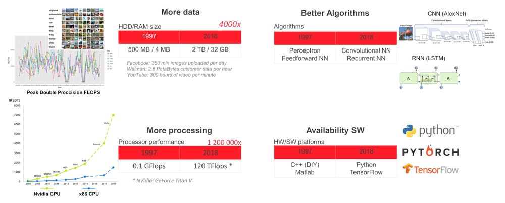
In the present state of technology we can train deep neural network (DNN) for a specific tasks like object and human face detection and recognition, speech recognition, language translation, games (chess, go, etc.), autonomous vehicle driving, sensor status monitoring and predictive machine maintenance decisions, evaluation of X-ray images in healthcare etc. For such specialized tasks, a DNN can reach or even exceeds human capabilities.
Why Use Artificial Intelligence on the Edge
For example, the modern building contains a lot of sensors, HVAC devices, elevators, security cameras, etc. connected to the internal network. For the security, latency or robustness reasons, it is more appropriate to run artificial intelligence tasks locally, on the edge of a local network, and send only anonymized data that are necessary for taking global decisions to the cloud.
Hardware on the Edge
To deploy DNN on the edge we need a device with enough computing power and simultaneously low power consumption. The current state of technology offers a combination of low power CPU and VPU accelerator (x86 CPU SBC+ Intel Myriad X VPU) or CPU + GPU accelerator (ARM CPU + Nvidia GPU).
The easiest way to start DNN is using UP Squared AI Vision X Developer Kit version B. It is based on UP Square SBC with Intel Atom®X7-E3950 processor with 8GB RAM, 64 GB eMMC, AI Core X module with Myriad X MA2485 VPU and USB camera with resolution 1920 x 1080 and manual focus. The kit is preinstalled with Ubuntu 16.04 (kernel 4.15) and OpenVINO toolkit 2018 R5.
Toolkit contains precompiled demo applications in /home/upsquared/build/intel64/Release and pre-trained models in /opt/intel/computer_vision_sdk/deployment_tools/intel_models. To see help for any demo application, run it in terminal with –h option. It is recommended to initialize OpenVINO environment before running demo application by command source /opt/intel/computer_vision_sdk/bin/setupvars.sh.
Besides UP Squared AI Vision X Developer Kit, AAEON also offers:
1.Myriad X MA2485 VPU based modules: AI Core X (mPCIe full-size, 1x Myriad X), AI Core XM 2280 (M.2 2280 B+M key, 2x Myriad X), AI Core XP4/ XP8 (PCIE [x4] card, 4 or 8x Myriad X).
2.BOXER-8000 series based on Nvidia Jetson TX2 module.
3.BOXER-8320AI with Core i3-6100U or Celeron 3955U processor and two AI Core X modules.
4.Boxer-6841M series with the motherboard for Intel 6th / 7th generation of Core-I or Xeon processor for socket LGA1151 and 1x PCIe [x16] or 2x PCIe [x8] slots for GPU with power consumption max. 250W.
Hardware for Learning
To train DNN we need high computing power. For example, on the ImageNet competition in 2012, the winning team used the convolutional neural network AlexNet. 1.4 ExaFLOP=1,4e6 TFLOP operations were required for learning. It took 5 to 6 days on two Nvidia GTX 580 GPUs, where each has the 1.5 TFLOP computing performance.The table below summarizes the theoretical peak performance of the hardware.
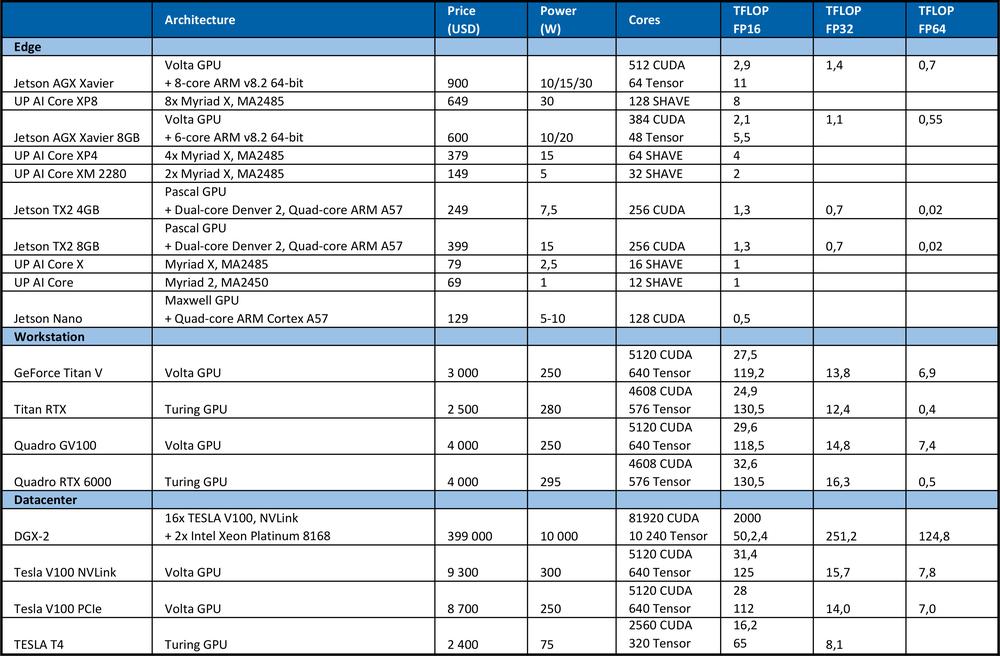
For comparison, the high-end Intel Xeon Platinum 8180 processor
●has 28 cores with 2 AVX-512 & FMA units per core
●AVX-512 turbo frequency 2.3GHz if all cores are active
●costs USD 10 000
It offers theoretical peak performance: # of cores * frequency in GHz * AVX-512 DP FLOPS/Hz * # of AVX-512 units * 2 = 2060.8 GFLOPS in double precision (DP) → 4.1216 TFLOPS in single (32-bit).
As you can see from the table above, GPU provides far more performance for neural networks learning. It is necessary to note that the number of operations per second is not the only parameter that affects learning performance. Factors as RAM size, the data transfer rate between CPU and RAM, GPU and GPU RAM or between GPU also influence the learning speed.
Software
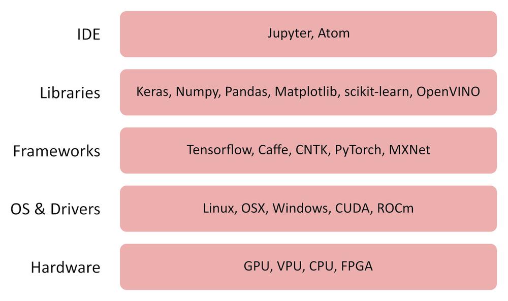
OpenVINO
The OpenVINO (open visual inference and neural network) toolkit is free software that allows quick deployment of applications and solutions that emulate human vision.
The OpenVINO toolkit:
●Uses CNN (convolution neural network)
●Can split computation between Intel CPU, integrated GPU, Intel FPGA, Intel Movidius Neural Compute Stick and vision accelerators with Intel Movidius Myriad VPUs
●Provides an optimized interface to OpenCV, OpenCL, and OpenVX
●Supports Caffe, TensorFlow, MXNet, ONNX, Kaldi frameworks
https://software.intel.com/en-us/openvino-toolkit, https://docs.openvinotoolkit.org
TensorFlow
TensorFlow is an open-source library for numerical computation and machine learning. It provides a convenient front-end API for building applications in Python programming language. However, the TensorFlow-generated application itself is converted to optimized C ++ code that can run on a variety of platforms such as CPUs, GPUs, local machine, a cluster in the cloud, embedded devices at the edge and the like.
Other Useful Software
Jupyter Lab / Notebook
https://jupyter.org/index.html
https://github.com/jupyter/jupyter/wiki/Jupyter-kernels
https://jupyterlab.readthedocs.io/en/stable
Keras
Pandas
MatplotLib
Numpy
How it Works
Simplified Neuron Model
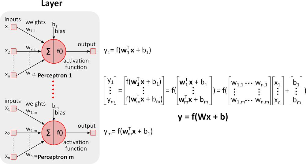
Simple neuron model – the perceptron was first time described by Warren McCulloch and Walter Pitts in 1943 and it is still the standard of reference in the field of neural networks.
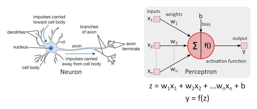
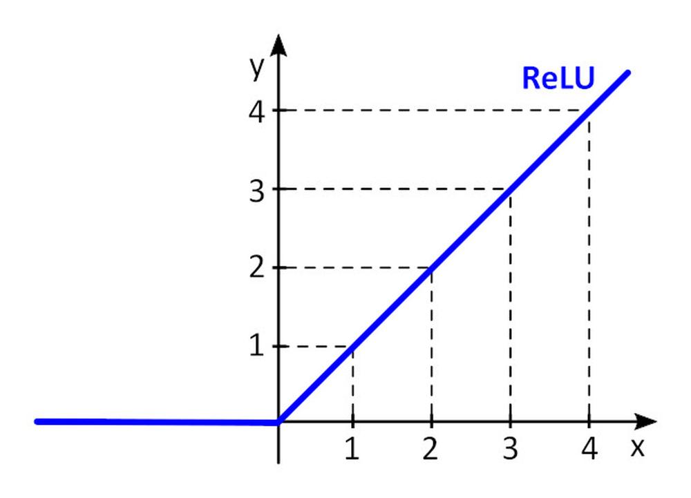
Activation function f () adds nonlinearity to perceptron. Without non-linear activation function in the neural network (NN) of perceptrons, no matter how many layers it had, it would behave just like a single-layer perceptron, because summing these layers would give you just another linear function. The most often used activation function is rectified linear unit – ReLU.
y = f(x) = max (0, x), for x < = 0, y = 0, for x ≥ 0, y=x

Inference (Forward pass)
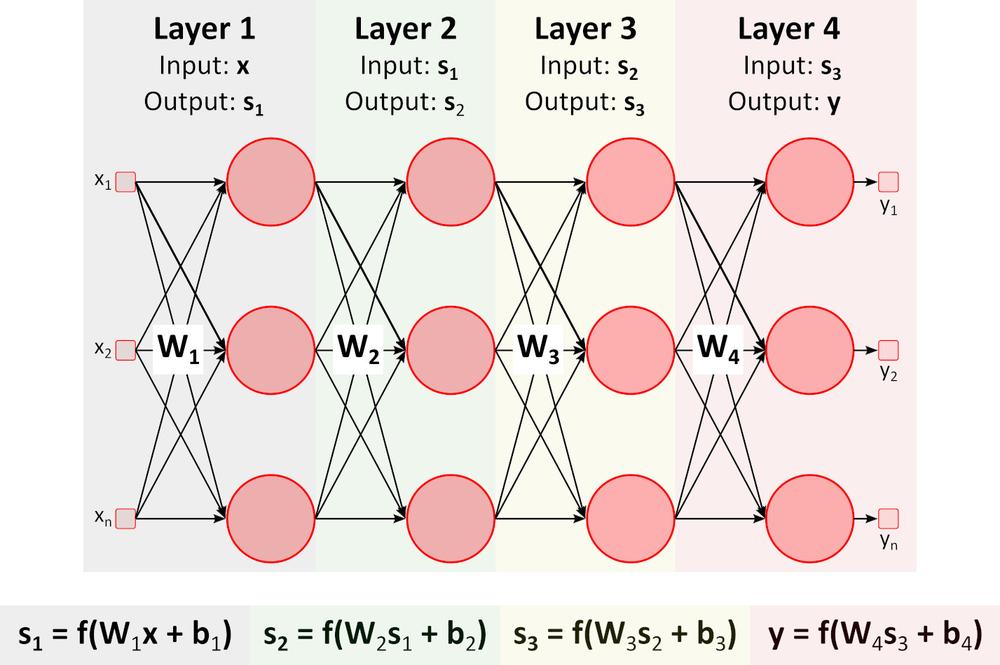
The figure above shows a deep neural network (DNN) because it contains multiple layers between input and output layers. As you can notice, DNN requires matrix multiplications and additions. Special hardware optimized for this task, such as GPU (graphics processing unit) and VPU (vision processing unit), is much faster than general-purpose CPU (central processing unit, processor) and has lower power consumption.
Learning (Backward pass)
Let’s say we want to teach DNN to recognize orange, banana, apple, and raspberry (object classes) in the image.
1. We prepare a lot of images of fruits above and divide it into the training set and validation set. The training set contains images and correct, required outputs for these images. DNN will have 4 outputs. The first output provides a score (probability) that fruit in the picture is orange, the second provides the same for a banana, etc.
2.We set initial values for all weights w_i and biases b_i. Random values are typically used.
3.We pass the first image through DNN. The network provides scores (probability) on each output. Let’s say that the first image depicts orange. Network outputs can be y= (orange, banana, apple, raspberry) = (0.5, 0.1, 0.3, 0.1). Network “says” that input is orange with a probability of 0.5.
4.We define a loss (error) function that quantifies the agreement between the predicted scores and the correct scores for each class. Function E = 0.5*sum (e_j) ^2, where e_j = y_j - y_real_j and j is number of images in training set is often used. E_1_orange = 0.5*(0.5-1)^2=0.125, E_1_banana =.0.5*(0.1-0)^2 = 0.005 E_1_apple = 0.5*(0.3-0)^2 = 0.045, E_1_raspberry = 0.5*(0.1-0)^2 = 0.005 E_1 = (0.125, 0.005, 0.045, 0.005)
5.We pass all the remaining images from the training set through DNN and calculate E (E_orange, E_banana, E_apple, E_raspberry) loss function value for the whole training set.
6.To modify all weights w_i and biases b_i for the next training pass (epoch), we need to know the influence of each parameter w_i and b_i to loss function for each class. If the increase of parameter value causes the increase of loss function value, we need to decrease this parameter and vice versa. But how to calculate required parameters increase or decrease?
Let’s try a simple example.
We have three points with coordinates (x, y): (1, 3), (2.5, 2), (3.5, 5). We want to find a line y = w.x + b for which loss function E = 0.5*sum (e_j) ^2 , where e_j = y_j – y_real_j, j=1, 2, 3 is minimal. To make task as simple as possible, let’s say that w=1.2 and we need to find optimal value for b only. We pick the initial value for b=0.
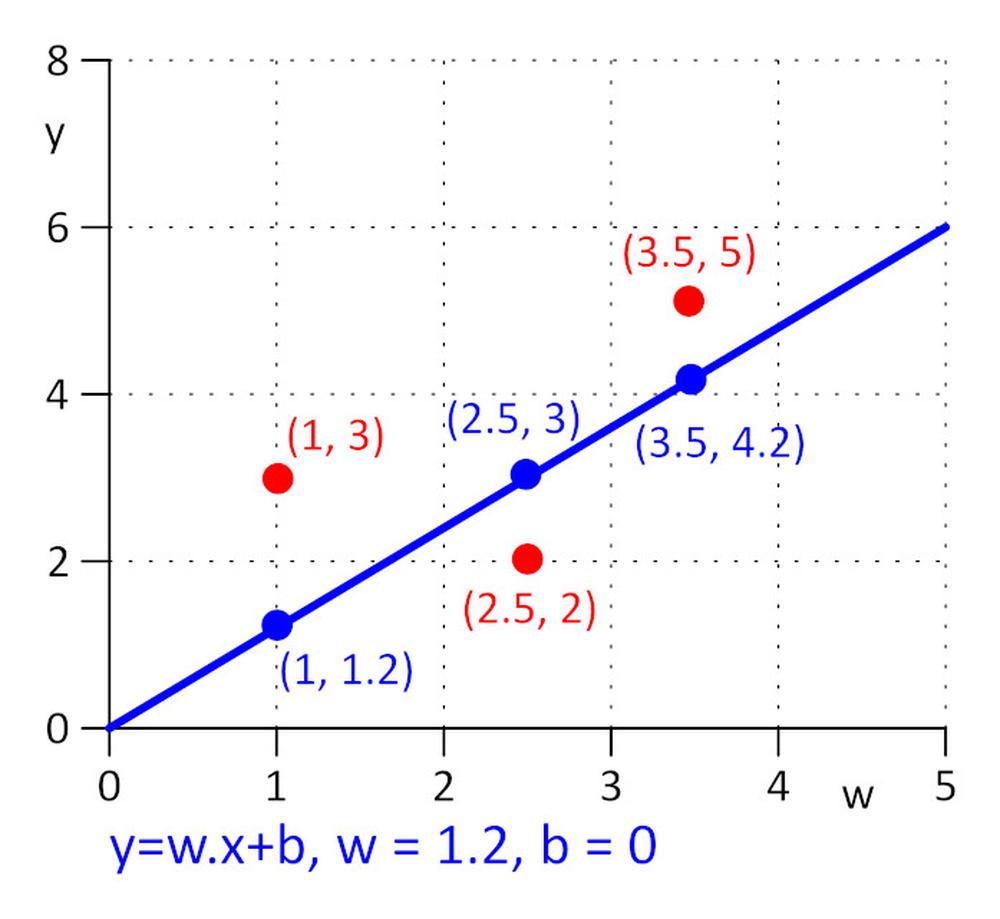
Let’s calculate loss function: E = 0.5*sum (e_j) ^2 = 0.5*(e_1^2 + e_2^2 + e_3^2), e_1=1.2*1 + b -3, e_2 = 1.2*2.5 + b – 2, e_3 = 1.2*3.5 + b – 5.
Loss function E is simple, we can find a minimum of E by solving equation: ∂E/∂b = 0. It is a compound function, to calculate ∂E/∂b we apply the chain rule.
∂E/∂b=0.5*((∂E/∂e_1)*(∂e_1/∂b) + (∂E/∂e_2)*(∂e_2/∂b) + (∂E/∂e_3)*(∂e_3/∂b)) = 0.5*(2*e_1*1 + 2*e_2*1 + 2*e_3*1) = (1.2*1 + b – 3) + (1.2*2.5 + b – 2) + (1.2*3.5 + b – 5) = 0 => b = 0.53333
In practice, where number of parameters w_i and b_i can reach a million or more, it is not practical to solve equation ∂E/∂b_i = 0 and ∂E/∂b_i = 0 directly, iterative algorithm is used instead of that.
We started with b = 0, next value will be b_1 = b_0 – η*∂E/∂b, where η is learning rate (hyper-parameter) and -η*∂E/∂b is step size. We stop learning when step size reaches the defined threshold, in practice 0.001 or smaller.
For η = 0.3, b_1 = 0.48, b_2 = 0.528, b_3 = 0.5328 and b_4 = 0.53328 and b_5 = 0.5533328. After 5 iterations the step size dropped to 4.8e-5 and we stop learning here. The value of b obtained by this algorithm is practically the same as the value obtained by solving the equation ∂E/∂b=0.
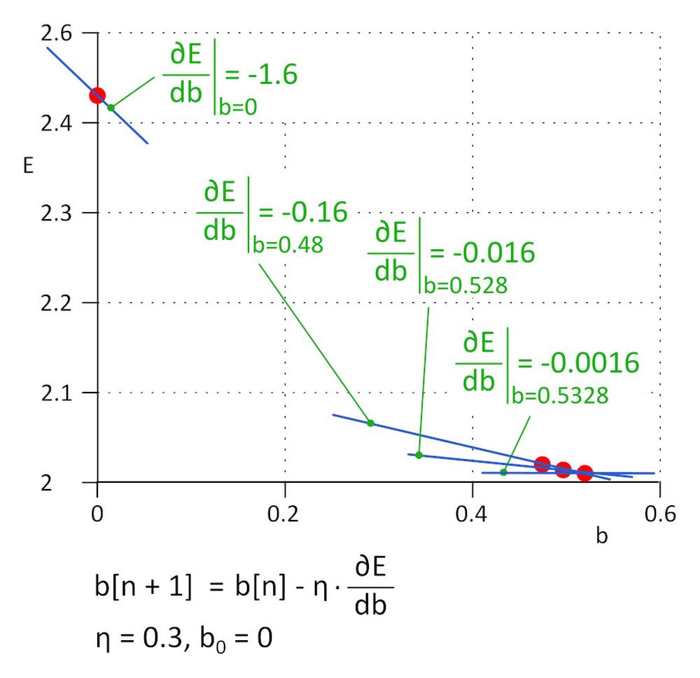
This method is called gradient descend.
Learning rate is an important hyper-parameter. If it is too small, it takes a lot of steps to find a minimum loss function; if it is high, the algorithm can fail. In practice, improved variants of an algorithm such as Adam are used.
7.We repeat steps 5 and 6 until loss function value decreases to the required value.
8.We pass the validation set through trained DNN and evaluate accuracy.
In the present time, DNN learning is a highly experimental work. Many DNN architectures are known, each of them is well suited for a particular range of tasks. Every DNN architecture has its own set of hyper-parameters that influence the behavior of DNN. Arm yourself with patience and the result will come soon.
For further information about AAEON products, please do not hesitate to contact us at aaeon@soselectronic.com
Do you like our articles? Do not miss any of them! You do not have to worry about anything, we will arrange delivery to you.


